SPIKESbind
  • Development Tool
  • Self-Assessment Tool
  • Quiz
  • -log Ki Table
  • Assumptions of the Model
-log Ki Table
Open in new window

Hypothetical ligands have been included in the model to increase its applicability.

Ligand A and Ligand B are examples of ligands that have marked differences in affinities (-log Ki values) for receptor subtypes (not evident with established ligands).

You may nominate affinities (-log Ki values) for Ligands C and D.

Competing
Ligand
-log Ki Value
M1 M2 M3 M4 M5
Established
Atropine 9.0 8.8 9.3 8.9 9.2
Pirenzepine 8.2 6.5 6.9 7.4 7.2
Methoctramine 6.7 7.7 6.0 7.0 6.3
Darifenacin 7.8 7.0 8.8 7.7 8.0
MT-3 6.7 5.9 6.0 8.1 6.0
S-Secoverine 8.0 7.9 7.7 7.7 6.5
Solifenacin 7.6 6.8 7.9 7.0 7.5
DAU-5884 8.9 7.1 8.9 8.5 8.1
Hypothetical
Ligand A 9.0 9.0 6.0 6.0 2.0
Ligand B 8.0 5.0 2.0 5.0 8.0
Ligand C * * * * *
Ligand D * * * * *
Assumptions of the Model
  1. All of the usual assumptions associated with Law of Mass Action that typically describe drug binding to receptors
    • All receptors are equally accessible to ligands.
    • All receptors are either free or bound to ligand - i.e. the model ignores any states of partial binding.
    • Neither ligand nor receptor are altered by binding.
    • Binding is reversible.

  2. Assumptions associated with competition binding studies
    • Only a small fraction of both the labelled and unlabelled ligands has bound, so the free concentration is virtually the same as the added concentration.
    • There is no co-operativity – binding to one binding site does not alter affinity at another site.
    • The experiment has reached equilibrium.
    • Binding is reversible and follows the law of mass action.

  3. Other model-specific assumptions
    • Analysis is conducted using % Specific Binding (no non-specific binding)
    • [3H-QNB] used in studies was << KA of 3H-QNB for receptors present, i.e. Cheng-Prusoff equation reduces to IC50 ≅ Ki for all competing ligands.

Self-Assessment Tool


Ligands
-log Ki Values
M1 M2 M3 M4 M5
1.
2.
3.
4.
5.
6.

The answer will be either one receptor subtype with a relative density of 100%, or more likely, a mixture of two receptor subtypes with relative proportions between 20% and 80% (in 10% increments).

SPIKES Approach

  • Shape
  • Position
  • IC50 values
  • Ki values
  • Elimination
  • Summation

An analysis of the shape of each competition binding curve within a binding study can provide an initial indication as to whether there exists one or more receptors in the cell/tissue. For example, if a competition binding curve is steep sigmoidal then the competing ligand is binding to a population of receptors for which it has a single affinity – this may be to one receptor or more receptors. On the other hand, if a competition binding curve is sigmoidal shallow or multiphasic, then this is clearly indicative that the ligand is binding to more than one receptor with different affinities – i.e. the cell/tissue contains more than receptor, although further analysis is required to identify the receptor subtypes present. Thus, analysis of the shape of competition binding curves is informative (may indicate whether the cell/tissue contains more than one receptor subtype) but not definitive (doesn’t identify the receptor subtype(s) present).

Determining the position of each of the competition binding curves is crucial to the identification of the receptors present in the cell/tissue. This is because the position of the competition binding curve is (at least in part) dependent upon the affinity of the competing ligand for the receptor(s) present. As explained further below, by identifying the position of the competition binding curve and completing appropriate analyses, it is possible to calculate the affinity of the ligand for the receptor(s) present and ultimately determine which receptor subtypes are present.

The position of steep sigmoidal and shallow sigmoidal competition binding curves is typically expressed in terms of an IC50 value – the concentration of competing ligand that reduces %Specific binding of the radioligand by 50% – and can be read directly from the competition binding curve or determined using computer-assisted analysis by fitting the data to a one-site binding model. Biphasic competition binding curves (the most common form of multiphasic binding, that contain two clear phases of binding separated by a clear point of inflection) will have two IC50 values – IC50(1) for the first phase of binding (at the lower concentrations of the competing ligand) and IC50(2) for the second phase of binding (at the higher concentrations of the competing ligand). IC50(1) and IC50(2) can be read directly from the competition binding curve or determined using computer-assisted analysis by fitting the data to a two-site binding model.

IC50 values are not a reliable measure of the affinity of the competing ligand for the receptor – this is because the IC50 value depends upon not only on the affinity of the competing ligand but also on the concentration and affinity of the radioligand. The higher the concentration of radioligand used, the higher the concentrations of competing ligand required to outcompete the radioligand and the higher the IC50 value. Nevertheless, IC50 values can be used to calculate the absolute affinity of the competing ligand for the receptor (Ki) present by applying the Cheng-Prusoff (1973) equation:
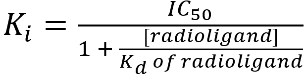
where
Ki = the affinity of the competing ligand for the receptor(s) present(the ‘i’ indicates the affinity value was determined from a competition (inhibition) binding study)

IC50 = the concentration of competing ligand that reduces radioligand binding by 50% (determined from the competition binding curve)

[radioligand] = the concentration of radioligand used in the competition binding study

Kd of radioligand = the affinity of the radioligand for the receptors – typically determined from a previously-completed saturation binding study

Application of the Cheng-Prusoff equation to generate Ki values (true measure of affinity) is appropriate for IC50 values generated from steep sigmoidal and biphasic competition binding curves, but not shallow sigmoidal competition binding curves. That is, although a single IC50 value can be readily derived from a shallow sigmoidal curve, it represents the binding of the competing ligand to at least two receptor subtypes with different affinities – so the single Ki value derived from the IC50 value of a shallow sigmoidal curve is a ‘composite Ki value’ which does not faithfully represent the true affinity of the competing ligand for either receptor subtype (Note though that the ‘composite Ki value’ will lay between the two true Ki values). Calculating the two true Ki values for a shallow competition binding curve requires fitting the data to a two site binding model (to generate two IC50 values) and using the Cheng-Prusoff equation (to convert each IC50 value into a Ki value).

From the Cheng-Prusoff equation, notice that if the [radioligand] used is very low (compared to Kd of radioligand) then the quotient [radioligand]/Kd of radioligand approaches zero, the value of the denominator approaches 1, and the Ki value approximates the IC50 value. That is, when the [radioligand] << Kd of radioligand then the visually-determined IC50 value (read directly from the competition binding curve) can be used as a good approximation of the Ki value for the competing ligand.

In SPIKESmate, the [radioligand] << Kd of radioligand, and thus the logIC50 values obtained directly from the competition binding curves can be used as a direct approximation of the affinity (logKi value) of the ligand for the receptor(s) present (i.e. no need to apply the Cheng-Prusoff equation).

As mentioned above, the Ki value is a measure of the affinity of the competing ligand for the receptor – it is often expressed as a –logKi value. The Ki value is determined by applying the Cheng-Prusoff equation to the IC50 values read/determined from the competition binding curve, as indicated above. The units of the Ki value are molar concentration, consistent with the idea that the Ki value is the concentration of ligand that will occupy 50% of receptors in the absence of any competing ligand. Thus, the lower the Ki value, the higher the affinity of the ligand for the receptor.

Comparison of the –logKi values obtained for a range of receptor-selective competing ligands in a competition binding study to their known –logKi values (obtained from competition binding studies using pure populations of recombinant human M receptor subtypes), together with a process of elimination and summation can be used to determine which M receptor subtypes are present in a cell/tissue.

The comparison involves determining the absolute difference between the single –logKi value obtained for a competing ligand in a cell/tissue to each of the known –logKi values for that competing ligand at each of the receptor subtypes (e.g. M1, M2, M3, M4 and M5). If for any of the comparisons, the absolute difference in –logKi values is  1.0 unit then it is highly unlikely that any of those receptor subtypes are present in the cell/tissue.

For example, a competition binding study determined that the –logKi value of MT-3 in a cell/tissue was 6.3. This value of 6.3 is then compared to the known –logKi values of MT-3 at M1, M2, M3, M4 and M5 receptors (6.7, 5.9, 6.0, 8.1 and 6.0, respectively) – providing absolute differences of 0.4, 0.4, 0.3, 1.8 and 0.3. Of these differences only the difference of 1.8 at the M4 receptor subtype is ≥ 1.0 unit. The conclusion drawn from the MT-3 competition binding curve (and –logKi value of 6.3) is that the cell/tissue does not contain a significant population of M4 receptors – i.e. the use of MT-3 has enabled us to eliminate the possibility that the cell/tissue contains M4 receptors. Although MT-3 has thus been useful in the example to eliminate the M4 receptor subtype, it does not provide any definitive additional information regarding which receptor(s) are present – there could be any combination of M1, M2, M3 and/or M5 receptors present. Determination of which receptor subtypes are present requires applying this elimination process to the –logKi values obtained visually to a range of other receptor-selective ligands (e.g. potentially to each of pirenzepine, methoctramine, darifenacin and S-secoverine) until all receptor subtypes have been eliminated except for the receptor subtypes present.

Only relatively rarely can the use of a –logKi value obtained from a single competing ligand successfully identify which receptor is present in a cell/tissue – that is, only in the instance where the competing ligand is highly selective for the single receptor present (e.g. MT-3 binding to a cell/tissue containing a pure population of M4 receptors, S-secoverine binding to a cell/tissue containing a pure population of M5 receptors or DAU-5884 binding to a cell/tissue containing a pure population of M2 receptors).

In the Elimination process, each different competing ligand may be able to eliminate one or more receptor subtypes as having been present within the cell/tissue. By using the information obtained from ALL the competing ligands (Summation), a concerted process of elimination should leave just those receptors that are present in the cell/tissue not being eliminated. Illustrations of how the SPIKES approach can be used to determine which receptors are present in a particular cell/tissue are presented in the worked Examples #1 - #7.

Competition Binding Curves
  • About
  • ⋅
  • Instructions
  • ⋅
  • Contact

Creative Commons 2018

Instructions

The Development Tool can be used to visualise how the shape and position of competition binding curves can be influenced by:

1.  the relative densities of receptor subtypes expressed by cells or tissues, and

2.  the affinities of ligands for the receptor subtypes.

The following instructions demonstrate how these changes in the shape and position of competition binding curves can be visualised using the Development Tool.

Firstly, you select which receptor subtypes are present in the cell or tissue of interest.

Within the Receptor window, select up to three receptor subtype combinations by clicking on the appropriate buttons below the name of the subtype. Once a particular subtype has been selected, the Relative Density (%) box appears immediately below.

If only one receptor subtype is selected, then the Relative Density (%) value will be 100.

If two receptor subtypes are selected, then the sum of their Relative Density (%) values must be 100, i.e. increasing the value of one will decrease the value of the other to maintain a total value of 100. The Relative Density (%) values can be changed by either by using the arrows for increments of 1%, or by typing in the desired value (0-100).

If three receptor subtypes are selected, then the combined value must again be 100. In this case, enter the receptor density values in order from left to right, i.e. start with the receptor subtype with the lowest number selected (e.g. M1) to the receptor subtype with the highest number (e.g. M5).

Once the first two receptor densities have been selected, the final density will automatically be calculated.

For example, if you wished to use a cell that expresses a combination of M2, M4 and M5 receptors in the relative proportions 20:30:50, respectively, then select the M2, M4 and M5 subtypes. In order, enter the values of 20% for M2 and 30% for M4. M5 will automatically be assigned a 50% density.

Secondly, you select which ligands you wish to use in the competition binding studies.

Within the Ligands window, use the drop down menu to select up to 6 ligands from a list of 8 Established ligands and 4 Hypothetical ligands.

Established ligands are ligands that have been used extensively in the past, and for which there are known -log Ki values (e.g. Atropine).

Hypothetical ligands, as their name suggests do not exist in the real world, but have been included in SPIKESbind to increase applicability.

There are 2 types of Hypothetical ligands - one type includes Ligand A and Ligand B, which have marked (but defined) differences in affinities for receptor subtypes.

The second type of Hypothetical ligand includes Ligand C and Ligand D, and these are ligands where you can assign (and change) a –log Ki value (affinity) for each receptor subtype. The assigned –log Ki values must be between 3 and 10 and may be changed by either using the arrows (increments of 0.1), or by typing in the desired value (3-10).

The ligands included in the drop down menu and their corresponding -log Ki values can be viewed in the '-log Ki Table' tab.

Lastly, once receptor subtypes and ligands have been selected, a plot of the specific binding % is displayed in real time within the Competition Binding Curves window.

By inserting the appropriate -log Ki values into the one-, two- or three-site binding models, accompanied by the selected subtype receptors, SPIKESbind will calculate the % specific binding values over the ligand range 10-12 - 10-2 M and will generate the Competition Binding Curves for viewing.

A feature of SPIKESbind is that any changes to the receptor subtype or the ligands selected will cause the Competition Binding Curves window to be dynamically updated in real time, to reflect the new values. For example, you can directly observe (in real time) changes in the shape and position of Competition Binding Curves caused by (1) altering the Relative Densities of receptor subtypes or (2) altering ligand affinity (use Ligands C (or D) to observe this effect).

In the Self-Assessment Tool, you choose up to 6 ligands (from the list of 12 Established and Hypothetical ligands) that you wish to use in a competition binding study. The Competition Binding Curves for these selected ligands are then displayed in the Competition Binding Curves window based on a receptor profile (the receptor subtypes and their relative densities) that has been randomly generated by SPIKESbind.

The task for you is to analyse the competition binding curves using the SPIKES approach, and deduce which receptor subtypes are present and their relative densities. The actual receptor profile can be revealed at any time by clicking the Reveal Subtype button.

Firstly, you select which ligands you wish to use in the competition binding studies.

From within the Ligands window, select up to 6 Ligands from a list of 8 Established ligands and 4 Hypothetical ligands. As indicated above, Established ligands are ligands that have been used extensively in the past, whereas Hypothetical ligands, as their name suggests, do not exist in the real world, and have been included in SPIKESbind to increase applicability.

There are 2 types of Hypothetical ligands - one type includes Ligand A and Ligand B, which have marked (but defined) differences in affinities for receptor subtypes.

The second type of Hypothetical ligand includes Ligand C and Ligand D, and these are ligands where you can assign (and change) a –log Ki value (affinity) for each receptor subtype. The assigned –log Ki values must be between 3 and 10 and may be changed by either using the arrows (increments of 0.1), or by typing in the desired value (3-10).

The ligands included in the drop down menu and their corresponding -log Ki values can be viewed in the '-log Ki Table' tab.

Secondly, the competition binding curves will appear for the selected ligands, showing the specific binding % over the ligand range 10-12 - 10-2 M.

The shape and position of the competition binding curves generated depends on which specific receptor subtypes are present and their relative densities (e.g. 30% M1 and 70% M2). The receptor profile is randomly selected by SPIKESbind from a defined bank of approximately 75 options.

The bank of 75 options is based on the premise (1) that there are 10 possible combinations involving two receptor subtypes (M1/M2, M1/M3, M1/M4, M1/M5, M2/M3, M2/M4, M2/M5, M3/M4, M3/M5 and M4/M5), and (2) that for each receptor combination there are 7 possible receptor density combinations (20/80, 30/70, 40/60/ 50/50, 60/40, 70/30 and 80/20) – giving a total of 70 options for two-receptor subtype combinations. This 70 options, together with another 5 options for pure receptor subtypes (100%), gives a grand total of 75 options from with SPIKESbind can choose to present. All 90%/10% and small incremental combinations have been omitted for your benefit as they cannot be reliably interpreted by eye.

Using the SPIKES approach to deduce which receptor subtypes are present and their relative densities. Your answer should be one of the 75 options.

Lastly, after you have worked out your answer, you may reveal the solution to validate your work.

You can reveal which receptor subtype population exists and their relative densities by clicking the Reveal Subtype button, and the answer will appear.

After viewing the solution, the ligands may be modified in the ligand table to view other competition binding curves, including the custom -log Ki values for ligands C and D, and the graph will dynamically update.

To generate a new question in the Self-Assessment Tool, click the Reset button and a new receptor subtype combination option will be randomly generated by SPIKESbind.

The Quiz Tool works off the same premise as the Self-Assessment tool, where any one question is randomly selected from a list of 75 options (i.e. up to two receptor subtypes with relative densities between 20-80%, using 10% increments).

However, the Quiz Tool is different from the Self-Assessment tool as the ligands used in the Competition Binding studies are pre-selected by SPIKESbind. In the Quiz Tool, SPIKESbind selects 5 ligands – 4 of which will be randomly selected from the list of 7 selective Established ligands (Pirenzepine, Methoctramine, Darifenacin, MT-3, S-Secoverine, Solifenacin and DAU-5884), and one Hypothetical ligand, either Ligand A or Ligand B. This provides the opportunity for over 500 different questions to be posed by the Quiz Tool – sufficient to gain expert proficiency in interpreting competition binding data.

Analyse the Competition Binding Curves using the SPIKES approach to solve which receptor subtypes are present, and what their densities are. Note that not all questions within the Quiz Tool can be answered by eye – for these questions you should be able to indicate which additional ligand(s) would allow the question to be answered unequivocally (and why).

Prior to commencing the quizzes, you may wish to read through the SPIKES examples to gain an insight into how to systematically approach solving competition binding data using the SPIKES approach.

Follow the instructions below to undertake the Quiz.

From the Quiz homepage, click the Start Quiz button, and the quiz will commence with the question appearing.

At the top of the page, you will notice the timer appear, counting up from 0 seconds until your answer is submitted. This allows for you to record the time spent evaluating each question, and over time you should be able to see your times improve. Once the quiz is complete you are taken to the answer review page.

The graph in question will appear on the right hand size, showing the 5 pre-selected ligands plotted with the randomised mixed receptor subtype combination.

Use this information to work out your solution (i.e. which receptor subtypes are present and their relative densities). Provided is a ‘SPIKES Approach’ table for you to help determine the answer. In this table you are able to view the list of ligands displayed in the graph, along with their corresponding -log Ki values, a drop down menu to determine the shape of the curve, a position textbox to enter information for the -logIC50 value, and checkboxes to eliminate receptor subtypes (i.e. apply the SPIKES approach).

Once you have completed your analysis, enter which receptor subtype(s) you believe to be present and their relative densities, using the checkboxes and drop down menus provided.

After you are happy with your answer, click the Submit button to head to the answer 'Review' page.

At the ‘Review’ page, "Correct!" or "Incorrect" will appear, as will the competition binding curve again. If you answered incorrectly, another graph will be displayed to view what competition binding curves your selection would have created. You have the option to Amend your Answers or to start a New Quiz.

About

SPIKESbind is an educational application to boost students' proficiency in interpreting competition binding data by providing self-development, self-assessment and quiz-me options.

Most drugs work by binding to specific receptors, which are large proteins typically expressed on the surface of cells.

The process of drug binding requires the existence of affinity (chemical forces of attraction) between the drug and receptor, and can be readily described by relatively simple mathematical relationships.

As drug binding is essential for drug action, pharmacology students need to have an advanced level of understanding of how changes in the affinity of a drug for a receptor can influence binding, and be able to readily interpret drug binding data.

SPIKESbind was created by Madeline King, Jason Gan, Robert Fernandez and Timothy Mennell; students of CITS3200: Professional Computing at the University of Western Australia 2017, under the guidance of Associate Professor Peter Henry.

Cheng Y. and Prusoff W.H. (1973) Relationship between the inhibition constant (Ki) and the concentration of an inhibitor that causes a 50% inhibition (I50) of an enzymatic reaction. Biochem. Pharmacol. 22: 3099–3108.

D'Agostino G, Condino AM, Gioglio L, Zonta F, Tonini M, Barbieri A (2008). Isolated porcine bronchi provide a reliable model for development of bronchodilator anti-muscarinic agents for human use. Br J Pharmacol. 154: 1611-8.

DeLean A, Hancock AA, Lefkowitz RJ (1982). Validation and statistical analysis of the computer modeling method for quantitative analysis of radioligand binding data for mixtures of pharmacological subtypes. Mol. Pharmacol. 21: 5–16.

Eglen RM, Nahorski SR (2000). The muscarinic M(5) receptor: a silent or emerging subtype? Br J Pharmacol. 130:13-21.

Eglen RM, Choppin A, Watson N (2001). Therapeutic opportunities from muscarinic receptor research. Trends Pharmacol Sci. 22:409-14.

Flanagan CA (2016). GPCR-radioligand binding assays. Methods Cell Biol. 132:191-215.

Hein P., Michel MC, Leineweber K, Wieland T, Wettschureck N, Offermanns S (2005). Receptor and Binding Studies. In: Dhein S., Mohr F.W., Delmar M. (eds) Practical Methods in Cardiovascular Research. Springer, Berlin, Heidelberg.

Hulme EC, Trevethick MA. (2010) Ligand binding assays at equilibrium: validation and interpretation. Br J Pharmacol. 161:1219-37.

Kenakin TP (2004) A Pharmacology Primer: Theory, Application, and Methods. First Edn. Elsevier Academic Press, San Diego, CA, USA.

Limbird LE, Motulsky H (2011). Receptor Identification and Charcterisation. Suppl. 20. Handbook of Physiology, The Endocrine System, Cellular Endocrinology. https://doi.org/10.1002/cphy.cp070104

Liu H, Hofmann J, Fish I, et al. (2018) Structure-guided development of selective M3 muscarinic acetylcholine receptor antagonists. Proc Natl Acad Sci U S A. 115:12046-12050.

Mansfield KJ, Liu L, Mitchelson FJ, Moore KH, Millard RJ, Burcher E (2005). Muscarinic receptor subtypes in human bladder detrusor and mucosa, studied by radioligand binding and quantitative competitive RT-PCR: changes in ageing. Br J Pharmacol. 144:1089-99.

Neubig RR, Spedding M, Kenakin T, Christopoulos A, International Union of Pharmacology Committee on Receptor Nomenclature and Drug Classification (2003). International Union of Pharmacology Committee on Receptor Nomenclature and Drug Classification. XXXVIII. Update on terms and symbols in quantitative pharmacology. Pharmacol Rev. 55:597-606.

Ohtake A, Saitoh C, Yuyama H, Ukai M, Okutsu H, Noguchi Y, Hatanaka T, Suzuki M, Sato S, Sasamata M, Miyata K (2007). Pharmacological characterization of a new antimuscarinic agent, solifenacin succinate, in comparison with other antimuscarinic agents. Biol Pharm Bull. 30:54-8.

Contact

Found a bug in our application?
Or simply wanted to give some feedback?
Please don't hesitate to let us know!

Peter Henry
Associate Professor
The University of Western Australia

Room 1.34, M Block,
School of Biomedical Sciences,
QEII Medical Centre

peter.henry@uwa.edu.au